THE LANGUAGE OF ALGORITHMS

The word "algorithm" can also be used to describe certain medical procedures. In this context, the algorithm is similar to a recipe, with ingredients and processes; however, it is the kind of recipe that specifies what to do under alternative conditions, e.g., cooking recipes that contain alternatives for high altitude cooking or ingredient substitutions. A medical algorithm may be used to describe a procedure or to prescribe a procedure. The algorithm may have a deterministic or a stochastic orientation, that is, emphasizing cause and effect or emphasizing the probabilities of various possible results or coincident conditions. An algorithm may also be presented as a time oriented flow or as an time- isolated procedure. Regardless of the variations in purpose or orientation, an algorithm is a succinct expression of the elements of the procedure and its language of expression should support the communication of the algorithm's meaning.

Inorganic chemistry provides a ready example of an algorithm; however, it is an imperfect model for medicine. In inorganic chemistry classes, we were taught a schema or algorithm for determining the constituents of an unknown sample. The first test divided the potential results into mutually exclusive sets. Each succeeding test subdivided the sets until all possibilities were either excluded or positively included. This algorithm worked because (within this carefully constructed set of problems) tests had been devised with clear, unequivocal results, e.g., pour in the reagent, if a precipitate forms, then X is present. Unfortunately, in medicine the tests and observables are seldom deterministic and frequently ambiguous. More than one cause can generate the observed results and one cause can generate different results. As a result, medical algorithms are generally less ambitious in both scope and precision than inorganic qualitative analysis.

Algorithms may be communicated in a natural language (such as English); however, they are well suited to presentations in a graphical language. An algorithm may be stated in any dialect (or set of symbols, definitions and connecting rules). Translations between some pairs of dialects are easy (can be accomplished by computer programs), while translations between other pairs currently require human intervention. This chapter addresses the connections among dialects, connections between dialects and presentations, and connections between presentations and situational needs.

DEFINITIONS

Several terms will be used in this chapter for which explicit definitions will be useful for ensuring a common understanding. These definitions will agree with those of many sources and may disagree with some; however, such agreement or disagreement is not significant. The definitions may be regarded as temporary, rather than universal.

PRESENTATION ELEMENTS

Presentations of an algorithm are based on the need that the algorithm must satisfy. These needs are dependent on the situation. The elements of time, scope, and determinism are discussed below.

Time

A physician who first diagnoses a patient's problem and plans to treat and monitor that patient over a long period has one view of time and process. A physician who is confronted with a patient in crisis, with possible past treatments and possible continuing effects of past medications (or withdrawal from same) has a different view of time and process. The first view of time in the process is dynamic and the second is static.

Scope

A physician who has been treating a particular patient for some time and has reached a decision point in the treatment has already eliminated a variety of potentially confounding influences on that decision. The physician with the new patient in crisis would like to consider the situation with the broadest scope, narrowing that scope purposefully and correctly. In these two examples, both views of time are static, but the desirable scopes differ.

Determinism

The inorganic chemistry qualitative analysis algorithm is deterministic; properly followed, its results are determined by the contents of the sample. Many medical conditions are insufficiently understood to permit detailed predictions. For example, the condition may respond to drug A or to drug B; however, predicting which will work for a given patient is essentially impossible. The algorithm may be to try the one to which most patients respond and observe the response. Alternatively, the algorithm might be to try the one with the fewest side effects or the lowest cost first. A stochastic orientation is seen when the decision depends strongly on the particular patient and the key variables are unobserved.

DIALECTS

The particular dialect of the language of algorithms that is selected to describe an algorithm should be based on the presentation desired. There are several standard dialects that may be used, each with its own characteristics. Various dialects (flow charts, Gantt charts, influence diagrams, and decision trees) for displaying general processes (or specifically algorithms) are discussed and illustrated below.

Flow Charts

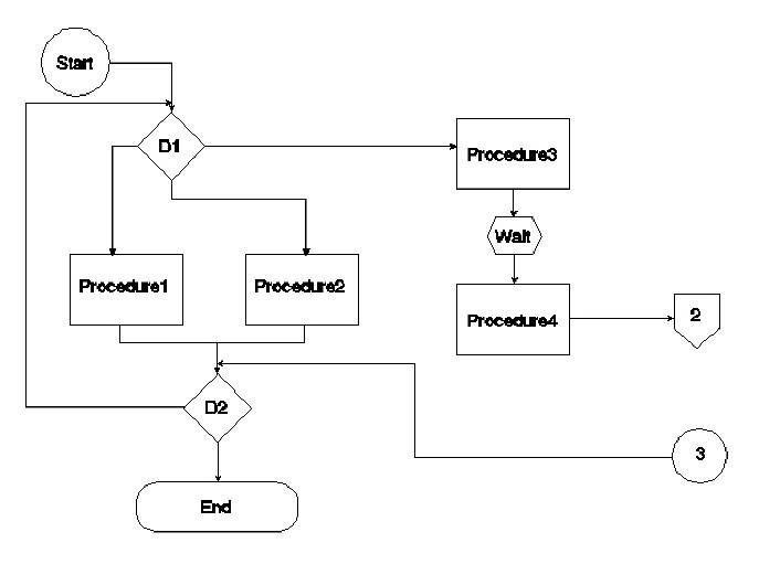
Flow charts emphasize procedural sequence, but not the passage of time. Various symbologies have been adopted as standards, e.g., computer program flow charts and chemical engineering flows. For medical algorithms, the standards are undefined. A representative flow chart is shown in Figure 1. The symbols used are defined as follows: a circle is an entry point, e.g., start point or connector from another page; a diamond is a decision procedure, with two or more exits; a rectangle is a procedure (with one exit), a hexagon is a waiting process; a pentagon is a connector to an off-page continuation; and a rounded box is an end point.

Time is poorly represented. Waiting (with specified times) can be represented; however, there is no easy way to compare the timelines of alternatives, nor is it easy to represent the duration of procedures. Flow charts also represent iterative processes well (note the arrow from decision D2 back to the entry to decision D1 in Figure 1); however, this further complicates conveying the passage of time. Flow charts are well suited for conversion to standard computer programs.

Gantt Charts

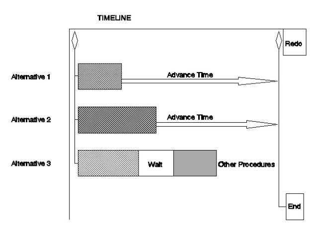
Gantt charts were specifically designed to represent processes with multiple procedures, each with varying durations. Their main use is in project management where simultaneous procedures are conducted. Gantt charts provide a graphical display that permits reduction of conflicting demands on resources and necessary waits for one procedure to be completed before another can be started. Changes to the standard conventions are required to display alternative procedures. Iterative procedures must either be explicitly expanded with replications of the parts or the charts must be defined as representing a single iteration, with reuse implied. The symbols of a Gantt chart include bars, with differing patterns representing differing procedures and length representing duration, and diamonds representing decision points. Figure 2 illustrates a modified Gantt chart. The Gantt chart emphasizes the duration of procedures well; however, complex processes may be difficult to display in a comprehensive and easily comprehendible fashion.

Gantt charts can be produced as fixed charts in various graphics programs. In addition, project management software generally allows for the production of active (automatically updated) Gantt charts. In active charts, the time line values can be modified as circumstances dictate. Project management software often implements more sophisticated active charts as well, either critical path method (CPM) or program evaluation and review technique (PERT) charts. These charts permit the modeling of more complex procedures; however, their orientation is toward minimizing the total time to complete a project, while avoiding over- commitment of resources, which is less generally the orientation of medical algorithms.

Influence Diagrams

Where flow charts and Gantt charts emphasize the relationships of decisions and procedures and the durations of procedures, respectively, influence diagrams emphasize the factors that are used in making the decisions. The symbology of influence diagrams includes ellipses, rectangles, rounded boxes, solid-line arrows, and dashed-line arrows. Ellipses represent uncertain events; double ellipses represent deterministic events, e.g., calculations; rectangles represent decisions; rounded boxes represent payoff tables; solid-line arrows lead to uncertain events and payoffs; and dashed-line arrows lead to decisions. (Clemen in Making Hard Decisions explains influence diagrams and decision trees very clearly [Clemen].) Influence diagrams represent sequence: predecessors in the diagram with respect to the arrows are also predecessors in a time sense; predecessors are defined as being resolved prior to their successors.

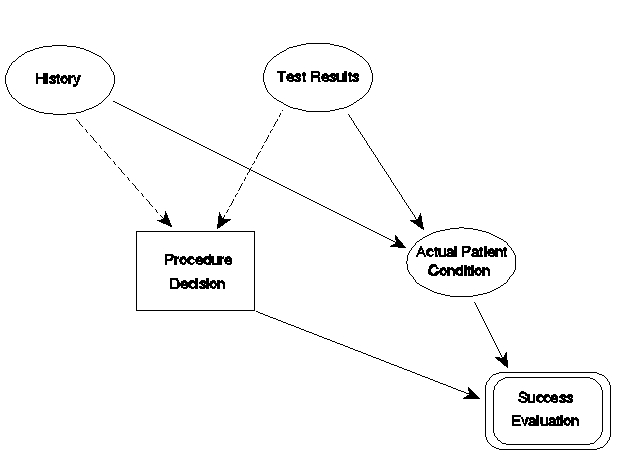
Figure 3 represents an influence diagram. In this diagram, the decision on the procedure to use is influenced by the patient's history and test results. These elements are uncertain in that each new patient will yield different sets of history and test results. The diagram says that the decision is conditioned on these results, not the actual patient condition; however, the history and test results are influenced by the patient's actual condition. The nature of the influence diagram dialect embodies conditional probabilities of correct test results, given the actual condition, and probabilities for the various values of actual condition; however, they are hidden within the symbols in the figure. The influence diagram omits the actual procedures: they are implied in the decisions. The final evaluation box is a payoff table that lists each combination of influences (here procedure choices and actual patient conditions) and the payoffs.

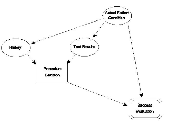
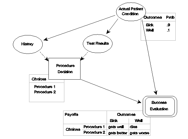
Figure 4 repeats the diagram, adding indications of the data behind three of the diagram elements. In this example, two choices are available in the procedures decision and two possible actual patient conditions are recognized. The data indicate that 90% of patients that arrive at this decision point are actually sick (probability = 0.9). The payoff table shows that Procedure 1 is very effective if the patient is actually sick: he or she gets well. However, if the patient is actually well, Procedure 1 kills him. Procedure 2 is less effective if the patient is sick: she gets better. However, if the patient is actually well, Procedure 2 only makes him or her worse. If the procedure decision were made blindly (without regard to history and test results), a decision to use Procedure 1 would have a 10% chance of killing the patient. However, as the use of Bayes Theorem of conditional probability confirms, the use of 90% accurate tests can decrease the risk to the neighborhood of 1%.

Influence diagrams concentrate on what goes into making a decision and allow calculations of the probabilities of various outcomes and their expected values. In addition, influence diagrams are well suited to programming as expert systems because they can represent systems without predetermined sequentiality. Such systems have internal sequences; however, the choice of the sequences to be followed depends on the data in a more fundamental fashion than normally seen in flow charts.

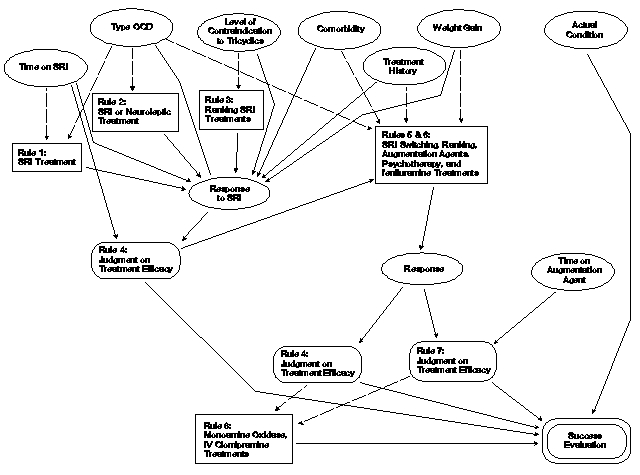
The lack of predetermined sequentiality is best explained with an illustration. Stein has implemented an algorithm for obsessive- compulsive disorder (OCD) as an expert system [Stein]. An abbreviated version has been converted to an influence diagram in Figure 5. In this diagram, eight "rules" are shown as decisions or payoffs. Each rule prescribes a set of actions or judgements that depends on various inputs. The rule is activated (or "fires") only under pre-set conditions concerning its inputs. Rules 1, 2, and 3 concern decisions on serotonin reuptake inhibitors (SRI). The patient's condition and history govern which rule fires and thus which decision set will be chosen. The patient's response is represented as an uncertain event that is influenced by the treatment decision and the condition and history. Two rules are represented as payoffs (4 and 7) because they are judgments about the response. (They might also have been represented as decisions, the proper choice depending on technicalities not germane here.) Rule 4 is influenced by the time on the SRI and the response. Rules 5 and 6 are combined in this diagram. The combined rule is invoked when a previous treatment is found to be inefficacious. It prescribes a new treatment, which generates a response that must be evaluated. One possible treatment is the addition of augmentation agents, in which case rule 7 is invoked. Rule 7 is influenced by the response and time on an augmentation agent. Figure 5 is not complete because several cycles of treatment changes may occur, requiring evaluations. However, a proper influence diagram contains no cycles. To create a complete influence diagram, several instantiations of rules 4 and 5 and the response are needed. The final decision, rule 8, represents a shift to a different class of treatments. The final payoff, success evaluation, is not present in the expert system, but is added to the influence diagram for completeness. Note that each of the potential end-state rules (4, 7, and 8) influence the evaluation, although only one will apply in any given case. The influence of the patient's actual condition on the payoff is represented; however, its influences on the various signs and symptoms are omitted to avoid excessive complexity in the figure.

Decision Trees

Decision trees are more familiar to most people than are influence diagrams; however, they are mathematically convertible to influence diagrams. Figure 6 shows the beginning of the inverse conversion for the influence diagram of Figure 3. The conditional probabilities of obtaining a particular history or test result, given the actual patient condition, have been reversed using Bayes' Theorem, yielding conditional probabilities of the actual patient condition, given the history and test results.

In influence diagrams, the actual choices are maintained in the background within the decision box, whereas in decision trees, the choices are explicitly shown. This explicitness comes at the cost of added complexity of the diagram, as shown in Figure 7. To maintain some simplicity, only two possible conditions for the patient are allowed: Cond 1 and Cond 2. The probabilities shown under each case may reflect probabilities of occurrence or historical percentage patterns at a given institution, or some other similar meaning, depending on the use to which the decision tree is to be put.

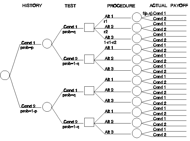
For the sake of illustration, assume that in patient histories Cond 1 occurs with frequency p (a fraction less than one) and (given only two choices) Cond 2 occurs with frequency 1-p. Similarly, assume that the test results have frequencies q and 1-q, respectively. The first two branchings of the tree represent the possible situations, with the probabilities for the four resulting branches being the products of the appropriate frequencies.

Note, that we could have represented the test results as being influenced by the histories to achieve a correlation between the two; however, in the original influence diagram, this correlation was induced by showing both histories and test results as being influenced by an unobserved actual patient condition. In applying these techniques to real situations, such questions comprise the essence of algorithm definition. In this instance, we only strive for verisimilitude.

In this illustration, there are three procedures, applied with frequencies r1, r2, and 1-r1-r2, irrespective of the patient history or test results. Finally, the actual patient condition, combined with the treatment choice, results in some payoff. Note the notation f(p,q), which indicates that the best guess at the probabilities for the true values for Cond 1 and Cond 2 are arrived at by computing the conditional probabilities, based on the information provided by the histories and test results. The value of the decision tree illustrated here would be in calculating the expected number of successes, failures, and partial successes, given the assumptions.

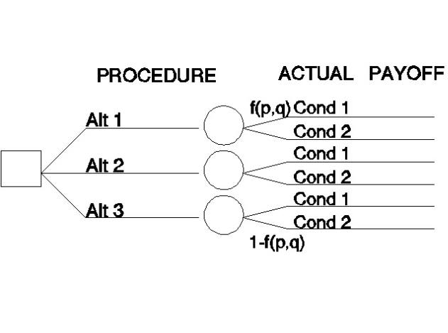
A variant is shown in Figure 8. The purpose of this decision tree is to aid in deciding on a procedure. The decision tree lays out all possible situations that might result from all possible decisions, along with the probabilities and the payoffs for each (not shown). The expected value of an alternative is the sum of the probabilities multiplied by the payoffs for the alternative. The preferred alternative is the one with the highest expected value (combination of high expectation of a positive result with low expectation of a negative result). Note that the influence of the history and test results is shown only indirectly in the probabilities of the actual patient (singular) condition.

There are computer programs that simplify the drawing of influence diagrams and their conversion to decision trees (and vice versa). These programs ask for the data input required and automatically calculate the values involved and aid in the discovery of proper probability choices.

EXPLICATING A REAL ALGORITHM

The algorithm shown in Figure 9 is part of a real (prototype) algorithm for treatment of schizophrenia. This algorithm is taken from the International Psychopharmacology Algorithm Project Report in the Psychopharmacology Bulletin [Zarate, et al.]. The text that amplifies the diagram is omitted; however, information found in the text will be used in recreating the algorithm in each of the four dialects.

Figure 9. Schizophrenia algorithm (NL=neuroleptic, ECT=electroconvulsive therapy) [Zarate, et al.].

Flow Chart for Schizophrenia

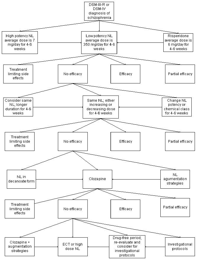
Figure 9 is not drawn in any of the standard dialects described here; however, it is easily convertible to a flow chart. Figure 10 contains the conversion of the algorithm's initial steps. The first two elements are the diagnosis procedure and the decision that the condition is schizophrenia. The third element makes the procedure decision of the algorithm explicit. Whichever procedure is chosen, it is evaluated after four to six weeks for efficacy. Treatment limiting side effects are addressed in a part of the algorithm not shown in the figure (represented by off-page connector 1). Similarly, the part of the algorithm that addresses maintenance treatment (when the treatment is at least partially effective) is not shown. The algorithm continues in Figure 10 with a procedure decision when the first treatment choice was not efficacious (another 4-6 weeks of the same treatment, a different dosage of the same drug, or change the drug). The algorithm continues in Figure 9, but the continuation is not shown in Figure 10 for brevity.

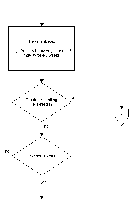
Neither the original algorithm diagram, nor the flow chart contains reference to possible interruptions to the treatment. A separate diagram is included in the algorithm; however, the mechanism for displaying its connection is inadequate. The diagram implies the question only arises after completing the 4-6 weeks of treatment in each case. A more realistic representation would replace each of the treatment rectangles with a treatment-test for side effects loop, as shown in the detail flow chart, Figure 11.

A further complicating factor is represented by comorbidity, the presence of other psychiatric disorders. The original algorithm also includes a separate diagram for this situation. This diagram should also be integrated; however, for purposes of this chapter, this complication is ignored, as the integration would be rather straightforward.

Note that there are two levels of "decisions" represented in the flow charts. One level is an evaluation of results, in which the results determine the flow. The other is a physician's choice among procedures that is dependent on complex of factors.

Gantt Chart for Schizophrenia

The schizophrenia algorithm also contains enough information to be converted to a Gantt chart (Figure 12). Only the portions of the algorithm that were shown in Figure 10 are included in the Gantt chart, again for brevity. Also, the contingent parts of the main-line algorithm (maintenance and side effects) are omitted because of their uncertainty with regard to the time line. Creative graphics might solve such problems.

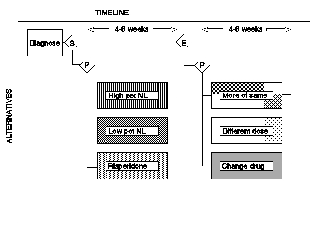
The diagnosis decision is represented by the diamond containing the "S" (for schizophrenia); the two procedure decisions are represented by diamonds containing a "P"; and the evaluation for efficacy decision is represented by the diamond containing the "E."

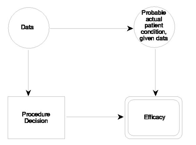
Influence Diagram for Schizophrenia

Figure 13 illustrates the conversion of the first two decisions of the schizophrenia algorithm to an influence diagram. The only portions of the original diagram that are explicitly represented are the precedence of the diagnosis decision to the treatment decision and the precedence of the treatment decision to the efficacy resolution. The influences that are diagrammed, however, are contained in the text that accompanies the diagram. The succeeding decision, relating to the efficacy of the treatment, is influenced by the treatment decision and the actual patient condition. Including the actual patient condition necessitates its influence on several of the uncertain events shown in Figure 13, such as medical history and symptoms.

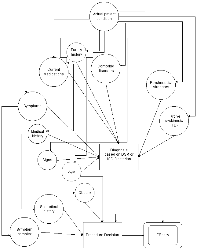
Note that in the influence diagram, the discovery of treatment limiting side effects follows the procedure decision, so all efficacy issues can be contained in a single symbol, regardless of whether discovered during the procedure or at its completion. The simple decision of the flow chart that represent determining the outcome of the diagnosis is included in the diagnosis procedure (of the influence diagram), which results in a diagnosis choice. The simple decisions that represent the efficacy tests are represented as uncertain events or as payoffs (as in this figure).

Table 1 illustrates the type of information that would be contained in the Efficacy payoff box of Figure 13. The list of possible actual conditions have been drawn from the actual algorithm, expanded to include some logical alternatives. The payoff entries represent the range of possible responses and not the actual responses. (The author is not a physician, nor an expert in psychiatry.)

ACTUAL CONDITION	PROCEDURE
ACTUAL CONDITION	High potency NL	Low potency NL	Risperidone
Not schizophrenic	side effects	no efficacy	side effects
Nonresponders	no efficacy	no efficacy	no efficacy
Intolerant	side effects	side effects	side effects
Excited psychosis, etc.	partial efficacy	partial efficacy	partial efficacy
Selective response A	efficacy	no efficacy	no efficacy
Selective response B	no efficacy	efficacy	no efficacy
Selective response C	no efficacy	no efficacy	efficacy
Selective response D	efficacy	efficacy	no efficacy
Selective response E	efficacy	no efficacy	efficacy
Selective response F	no efficacy	efficacy	efficacy
Typical	efficacy	efficacy	efficacy

Decision Tree for Schizophrenia

Whether the influence diagram is to be converted to a decision tree or solved directly, there are several steps required to reduce it to the situation where a decision is being evaluated. In this instance, we will evaluate the first procedure decision, using the influence diagram of Figure 14. The operative fact is the actual (total) patient condition, which has been estimated through the various tests and the diagnosis. The best estimate of the set of probabilities of the possible actual patient conditions is, therefore, the conditional probabilities of those conditions, given the various data. When these probabilities are adjudicated against the procedure choices, the expected efficacy matrix can be computed.

This reduced influence diagram is converted to a decision tree, illustrated in Figure 15. Conditional probabilities for the various actual conditions have been invented, as shown in the figure. Further, the effects have been assigned the numerical scores of 100 for full efficacy, 50 for partial efficacy, 0 for no efficacy, and -50 for side effects. These scores are multiplied by the probabilities to produce numerical payoffs, as shown.

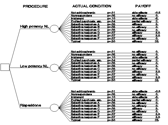
One product of decision trees is the scoring of the decisions. In this case, the sum of the scores for high potency neuroleptic (NL) is 31.5; for low potency NL, the score is 36.5; and, for risperidone, the score is 31.5. The low potency NL would be the choice here. (Note that this choice is an artifact of selecting "no efficacy" as opposed to "side effects" as the response for the "not schizophrenic" condition for this procedure and has no medical significance.) The scoring here has been strictly based on benefits; however, trivial modifications can produce cost scorings for cost/benefit analyses. Costs might represent only the monetary costs for drugs and physician fees or might include such factors as the cost of the patient's time.

The complete decision tree (or influence diagram) for schizophrenia is more complex than is shown here; however, the concept of creating the diagrams should be clear. The available commercial software allows for solving very complex diagrams with no user effort. The effort required is for the construction of the diagram to represent the algorithm correctly. Various probability distributions can be represented and tested. In addition, the testing process allows for re-examination of assumptions regarding the correct probabilities. For example, with no specific patient, the probabilities for each of the outcomes over all possible treatment patterns should result in the observed distribution of patient outcomes (efficacy, partial efficacy, side effects, etc.). If the results differ from the historical results, then either the internal probabilities are incorrect; the algorithm is not constructed properly; actual practice differs from the algorithm; or some combination of these possibilities obtains.

CREATING ALGORITHMS

Figure 16 shows the general form (influence diagram) of a multi- step algorithm (expanded from Figure 6). Each step consists of a procedure decision based on the available data. The actual condition is influenced by the procedure decision and the actual condition from the previous step. (In the first step, the actual condition is shown with its arrows to the data reversed using Bayes Theorem.) The apparent efficacy of that step is influenced by the actual condition and the chosen procedure and becomes the basis for the next step. In the last step, the apparent efficacy is replaced with success evaluation.

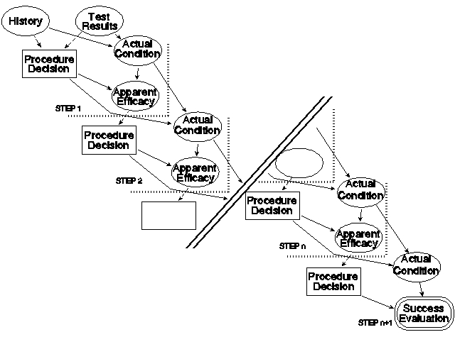
As with many things, the devil is in the details and so is the value. This structure is useful for the creation of a particular algorithm because it organizes the details: what are the data that influence the procedure decision at a given step? What are the procedure choices for that step? What are desiderata for the choices? What are the particulars of the procedures? What are the possible outcomes? What patient conditions influence those outcomes? What are the various probabilities? What are the research data upon which these details are based?

An initial set of data elements is presented in the following tables. It is expected that several applications to real algorithms will be required to ensure that all elements are included and that all possible relationships are considered.

Table 2 displays the data that are needed for each influence diagram decision (each of which will also be a flow chart decision). The "idnum" is a convenient short reference for use among the various components of the diagrams, whereas the label contains the content displayed in the symbol and aids in understanding the diagram. The choices are the various procedures that can be specified by this decision; the conditions are the desiderata for the choices; and the references specify the citation numbers. For flow charts, the idnums listed in the choices provide the connections to the proper procedure symbols of the flow chart. (Note that for some flow chart decisions, the procedure precedes the decision. An example is a diagnosis procedure followed by the diagnosis decision, used to control the flow in the diagram. These two flow chart symbols would be combined into a single influence diagram decision.) For influence diagrams (and decision trees), the procedure choices are contained in the decision symbol, thus the list of symbols directly influenced by this decision is provided by the connections list.

Element	Contents	Example Values
Idnum	Identifying number	d1, d2, ...
Label	short name	Procedure 1?
Descrip	description	1st procedure choice
Choice	action choices	{p1, p2, p3}
Cond	respective choice conditions	{ , , }
Ref	respective idnum(s) of reference(s)	{r1, r3, {r8, r9}}
Connect	idnum of successor(s) in influence diagram and decision tree dialects	{e1}, {u1, u3}, {d6} ...

Table 3 displays the data that are needed for each flow chart procedure (and contained in each influence diagram decision). The idnum identifies the flow chart symbol and is referenced in the appropriate influence diagram decision symbol. (Complex procedures involving sub-procedures and internal decision are special cases that may be initially coded as a single procedure and later resolved into detailed components.) The duration is required for Gantt charts. The connection idnums are required for flow charts. (In influence diagrams, the connections are provided by the decision symbol; however, care will be required to ensure consistency. All procedures specified by a single decision must have the same set of successors.

Element	Contents	Example Values
Idnum	Identifying number	p1, p2, ...
Label	short name	Low Pot NL
Descrip	description	Low potency NL, average dose is 350 mg/day
Dur	duration	4-6 weeks
Connect	idnum of successor(s)	{d1}, {d1, d2}, ...
Ref	idnum(s) of reference(s)	{r1}, {r1, r3, r8}, ...

Table 4 displays the data that are needed for each influence diagram uncertain event and flow chart decisions that represent flow control based on the value of a variable. The principal data required here are the possible outcomes and their probabilities or fractional distributions. Other elements are the successor events (influenced decisions and other uncertain events for influence diagrams) and procedures branched to for flow charts and appropriate references.

Element	Contents	Example Values
Idnum	Identifying number	u1, u2, ...
Decision	flow chart decision	'yes' or 'no'
Label	short name	Comorbid Psychosis
Descrip	description	Level of concurrent psychosis
Outcome	list of outcomes	{psychosis, moderate psychosis, no psychosis}
Prob	respective probabilities or distribution of outcomes	{ 0.1, 0.3, 0.5}
Ref	respective idnum(s) of reference(s)	{r1} {r3, r8, r9}, ...
Connect	idnum of successor(s)	{d1}, {d1, u2}, ... or {p3, p7, p8} for decisions

Table 5 displays the data that are needed for each influence diagram evaluation event and flow chart decisions that represent flow control based on the value of a variable. The principal data required here are the payoff values contained in the table of the possible outcomes versus choices from decisions. Other elements are the successor events (influenced decisions and other uncertain events for influence diagrams) and procedures branched to for flow charts and appropriate references.

Element	Contents	Example Values
Idnum	Identifying number	e1, e2, ...
Decision	flow chart decision	'yes' or 'no'
Label	short name	Success
Descrip	description	Table of degree of success results
Payoff	table of payoffs and reference idnums	{(choice1, outcome1: payoff11, r2), (choice1, outcome2: payoff12, r12), ... (choice2, outcome1: payoff21, r1), (choice2, outcome2: payoff22, r16), ... (choicen, outcomem: payoffnm, r1)}
Connect	idnum of successor(s)	{d1}, {d1, u2}, ... or {p6, p12, p20}

Table 6 displays the data needed for connecting the citation numbers (idnum) to the proper references. It also includes a short description of the relevant contents of the citation.

Element	Contents	Example Values
Idnum	Identifying number	r1, r2, ...
Label	short name	Bibliographic reference
Descrip	description	Relevant finding

The data contained in these tables are not new (except for the idnums for symbol connections and, perhaps, the statistics on outcomes). They are all contained in any complete description of an algorithm. What is different is the organization.

The best presentation of an algorithm depends on the use to which it will be put. The best presentation may also depend on the current state of knowledge. Stein, Patterson and Hollander discuss a classification of domains of knowledge with respect to suitability for expert systems. They divide knowledge into the domains based on data and rules, segmenting both data and rules as to whether little or much is known. Each of the four resulting domains provides differing challenges in creating expert systems and, by extension, differing challenges for any particular dialect. The advantage of creating a complete tabular description of an algorithm is that the presentation decision need not be made before knowing what the ultimate use will be, nor before ascertaining the true state of knowledge upon which the algorithm will be based.

CONCLUSION

Four dialects of the language of algorithms have been presented and discussed in this chapter. The data required for a complete description of an algorithm, in any of the four dialects, have been collected and organized into a set of tables. Flow charts, as their name indicates, emphasize the flow of the algorithm, where the branches are and what are the activities encompassed in the algorithm. Gantt charts emphasize the duration of activities and any time overlaps (alternative or simultaneous procedures). Influence diagrams emphasize the factors that must be considered in making decisions, including prior decisions. Decision trees emphasize the range of options considered in a decision and their consequences through subsequent decisions. Both influence diagrams and decision trees can be "solved" or computationally analyzed. Each dialect provides useful information about the algorithm, addressing different presentation needs for a prospective user of the algorithm; however, no dialect satisfies all possible needs. Medical algorithms are created as compact descriptions of procedures for solving medical problems. Initial algorithms may be descriptive, rather than prescriptive, as in the first decision tree example. Analysis of descriptive algorithms can lead to improvements based on the mathematics of expected values or may lead to better focused research, which will lead to improved algorithms.

Prescriptive algorithms represent the best available advice on treating medical problems. However, for prescriptive algorithms to be effective, they must be used. At least two conditions must be met for algorithms to be used: their existence must be communicated to the potential users and the algorithms must be understandable. A third condition increases the likelihood of use: the form of the algorithm (its language dialect) should be directly applicable to the problem at hand. Talented and creative practitioners can reformulate algorithms; however, physicians under the press of time and those of a less creative bent may find this more than they can handle.

Clearly, the preferred option is not to present an algorithm in only one dialect, but to present the algorithm simultaneously in all dialects, with the choice of dialect for using being left to the physician using the dialect. This option is not a simple option currently, as the translation from the dialect most comfortable to the creator(s) of an algorithm requires manual intervention. Commercial software packages permit algorithms to be constructed for presentation as both influence diagrams and decision trees. The extension of such a software package to include flow charts and Gantt charts, while not a trivial matter, would be very useful. Further, the commercial software obviously provides the options for modifying the structure, needed for constructing the algorithm; however, these options are not desirable for general users of the algorithm and add to the apparent complexity. An additional desirable modification would be the facility of producing a "run time" version of the software that only includes switches for the dialect changes and a method for introducing the data for a particular patient, obtaining customized results. Until such software is available, production of each algorithm in each dialect is must be accomplished manually.

REFERENCES

Robert T. Clemen, Making Hard Decisions: An Introduction to Decision Analysis. Duxbury Press, Belmont, CA, 1990.

Saul I. Gass and Carl M. Harris, eds. Encyclopedia of Operations Research and Management Science. Kluwer Academic Publishers, Boston, 1996.

Hartley D. S. III. "The language of algorithms." In: Fawcett, J.; Stein, D. J.; Jobson, K.O., eds. Textbook of treatment algorithms in psychopharmacology. New York: John Wiley & Sons, 1999:15-31.

Dan J. Stein, Robert Patterson and Eric Hollander, "Expert Systems for Psychiatric Pharmacotherapy," Psychiatric Annals; 24: 1 / January 1994.

Carlos A. Zarate, Jr., et al., "Algorithm for the Treatment of Schizophrenia." Psychopharmacology Bulletin, Vol. 31, No. 3, 1995, pp 461-467.

If you arrived here using a keyword shortcut, you may use your browser's "back" key to return to the keyword distribution page.

Page Last Updated: Sunday, 04 February 2024 12:03 EDT, © 1999, 2002, 2005, 2006, 2008, 2012, 2016, 2024

PROJECT: THE LANGUAGE OF ALGORITHMS

(a later version appears as a chapter in a book edited by Fawcett, Stein, and Jobson)

Dean S. Hartley III